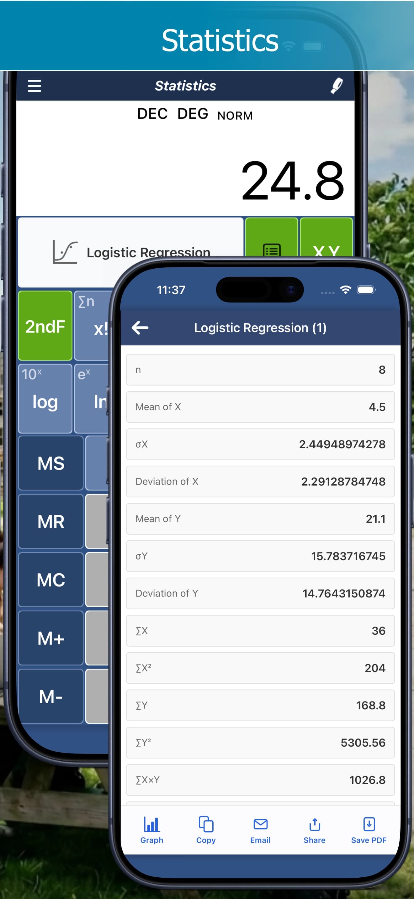
Statistics Calculator Guide: Descriptive Stats and 10 Regression Models

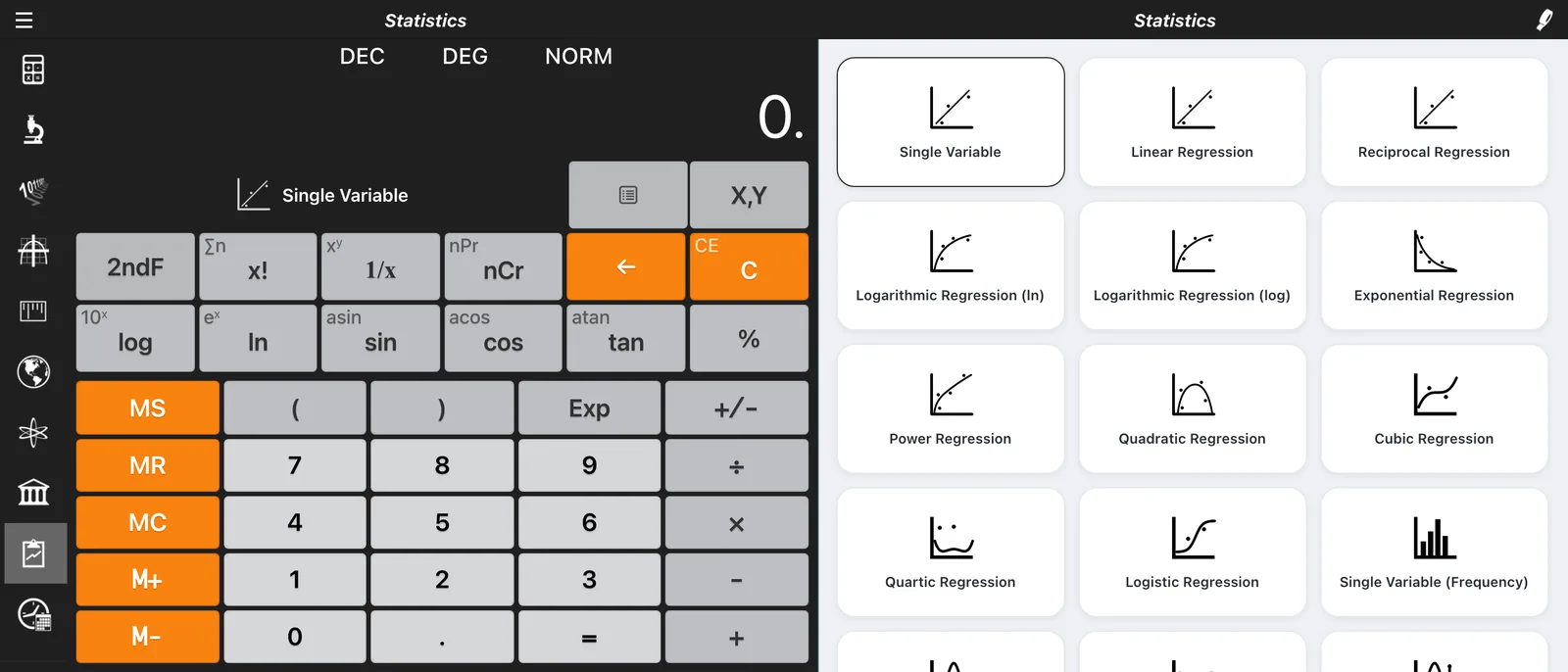
Calc Pro's Statistics Calculator transforms your device into a powerful data analysis tool. Whether you're a student, researcher, or business professional, this guide covers everything from basic descriptive statistics to advanced regression analysis.

Overview

The Statistics Calculator provides:

• Descriptive statistics (mean, median, quartiles, skewness, kurtosis and more)
• 10 regression types
• Probability distributions, confidence intervals and hypothesis tests
• Graphs of your data, plus PDF and e-mail export

In the iPhone & iPad app, features marked Pro Premium below unlock with the in-app purchase.

The Interface

Data Entry

Enter your data points using:

• The number pad
• The "Add" button to input each value
• Optional X-Y pairs for regression

Statistics Display

View calculated statistics:

• Central tendency measures
• Dispersion measures
• Regression coefficients

Regression Type Selection

Choose from 10 regression models:

• Linear (y = a + bx)
• Logarithmic, natural log (y = a + b·ln(x))
• Logarithmic, base 10 (y = a + b·log(x))
• Exponential (y = a·bˣ)
• Power (y = a·xᵇ)
• Reciprocal (y = a + b/x)
• Quadratic (y = ax² + bx + c)
• Cubic (y = ax³ + bx² + cx + d) — Pro Premium
• Quartic (y = ax⁴ + bx³ + cx² + dx + e) — Pro Premium
• Logistic (y = c / (1 + a·e⁻ᵇˣ)) — Pro Premium

Descriptive Statistics

Central Tendency

Mean (Average)

The sum of all values divided by the count:

Mean = Σx / n

Example: For data [2, 4, 6, 8, 10]

• Sum = 30
• Count = 5
• Mean = 6

Median

The middle value when data is sorted:

For odd count: Middle value

• [1, 3, 5, 7, 9] → Median = 5

For even count: Average of two middle values

• [1, 3, 5, 7] → Median = (3 + 5) / 2 = 4

Mode

The most frequently occurring value:

• [1, 2, 2, 3, 4] → Mode = 2
• Some datasets have no mode or multiple modes

Dispersion

Range

The difference between maximum and minimum:

Range = Max - Min

Example: [5, 10, 15, 20, 25]

• Range = 25 - 5 = 20

Variance

Average of squared deviations from the mean:

Population Variance:

σ² = Σ(x - μ)² / N

Sample Variance:

s² = Σ(x - x̄)² / (n - 1)

Standard Deviation

Square root of variance:

σ = √(Σ(x - μ)² / N)  [population]
s = √(Σ(x - x̄)² / (n-1))  [sample]

Interpretation:

• Low SD = data clustered near mean
• High SD = data spread out

Summary Statistics

Statistic	Symbol	Description
Count	n	Number of data points
Sum	Σx	Total of all values
Mean	x̄	Average value
Median	Med	Middle value
Mode	Mo	Most frequent value
Min	Min	Smallest value
Max	Max	Largest value
Range	R	Max - Min
Variance	s²	Spread measure (squared)
Std Dev	s	Spread measure
Sum of Squares	Σx²	Sum of squared values

Regression Analysis

Regression finds the best-fit line or curve through your data points.

Linear Regression (y = a + bx)

The most common regression type. Finds the straight line that best fits the data.

Coefficients:

• a (intercept): y-value when x = 0
• b (slope): Change in y per unit change in x

Example: Sales vs. Advertising

Advertising ($1000s)	Sales ($1000s)
1	5
2	8
3	10
4	14
5	16

Results:

• a (intercept) ≈ 2.2
• b (slope) ≈ 2.8
• Equation: y = 2.2 + 2.8x
• Interpretation: Each $1000 in advertising yields $2800 in sales

Correlation Coefficient (r)

Measures the strength of linear relationship:

r value	Interpretation
+1.0	Perfect positive correlation
+0.7 to +0.9	Strong positive
+0.4 to +0.7	Moderate positive
+0.1 to +0.4	Weak positive
0	No correlation
-0.1 to -0.4	Weak negative
-0.4 to -0.7	Moderate negative
-0.7 to -0.9	Strong negative
-1.0	Perfect negative correlation

Coefficient of Determination (r²)

Percentage of variance explained by the model:

• r² = 0.81 means 81% of variation is explained
• Higher r² = better fit

Logarithmic Regression (y = a + b·ln(x))

Best for data that increases rapidly then levels off.

Use cases:

• Learning curves
• Diminishing returns
• Growth that slows over time

Example: Learning Time

Practice Hours	Skills Score
1	40
5	65
10	75
20	82
50	90

A logarithmic fit captures how improvement slows with more practice.

Calc Pro also offers a base-10 version, y = a + b·log(x), which fits the same shape of data.

Exponential Regression (y = a·bˣ)

Best for data showing exponential growth or decay. b is the growth factor for each unit of x: above 1 the data grows, below 1 it decays.

Use cases:

• Population growth
• Compound interest
• Radioactive decay

Example: Bacteria Growth

Hours	Colony Size
0	100
2	180
4	320
6	580
8	1040

Exponential regression reveals the doubling time.

Power Regression (y = a·xᵇ)

Best for data where variables have a power relationship.

Use cases:

• Allometric scaling in biology
• Physics relationships (distance = ½at²)
• Economic production functions

Example: Area vs. Diameter

Diameter	Area
1	0.79
2	3.14
3	7.07
4	12.57

Power regression confirms A ∝ d² relationship.

Reciprocal Regression (y = a + b/x)

Best for hyperbolic relationships.

Use cases:

• Inverse relationships (speed vs. time)
• Asymptotic behavior

Quadratic Regression (y = ax² + bx + c)

Best for parabolic data patterns.

Use cases:

• Projectile motion
• Optimization problems
• U-shaped relationships

Example: Profit vs. Price

Price ($)	Units Sold	Revenue
5	100	500
10	80	800
15	60	900
20	40	800
25	20	500

Quadratic regression finds the optimal price point.

Cubic and Quartic Regression — Pro Premium

• Cubic: y = ax³ + bx² + cx + d
• Quartic: y = ax⁴ + bx³ + cx² + dx + e

Higher-order polynomials fit curves with more bends, such as data that rises, dips and rises again. Use them with care: with only a few data points, a quartic will fit almost anything without explaining it.

Logistic Regression (y = c / (1 + a·e⁻ᵇˣ)) — Pro Premium

Best for S-shaped growth that levels off at a maximum, c.

Use cases:

• Population growth with limited resources
• Product adoption over time
• The spread of information or disease

Probability Distributions — Pro Premium

The Distributions calculator finds probabilities without looking anything up in a table:

Distribution	You enter	You get
Normal	Mean, Std Dev, X Value	z-Score, P(X ≤ x), P(X ≥ x)
Inverse Normal	Mean, Std Dev, Probability	The x value for that probability
Binomial	Trials (n), Success Prob., Successes (k)	P(X = k), P(X ≤ k), P(X ≥ k)
Poisson	Mean (λ), Events (k)	P(X = k), P(X ≤ k), P(X ≥ k)
t-Dist	Degrees of freedom, t Value	P(T ≤ t), P(T ≥ t), two-tail p
Chi-Square	Degrees of freedom, χ² Value	P(X ≤ x), P(X ≥ x)

Confidence Intervals — Pro Premium

Estimate a population mean from a sample:

• Z interval when the population standard deviation (σ) is known
• t interval when it isn't

Enter the sample mean, standard deviation, sample size and confidence level. Calc Pro shows the critical value, margin of error, and the lower and upper bounds of the interval.

Hypothesis Tests — Pro Premium

Test a claim about a mean:

• 1-Sample Z and 1-Sample t: compare a sample mean with a hypothesized mean
• 2-Sample t: compare the means of two samples (enter the mean, standard deviation and size of each)

Calc Pro reports the z or t statistic so you can decide whether to reject the null hypothesis.

Frequency Data — Pro Premium

Single Variable (Frequency) lets you enter each value once with how many times it occurs, instead of typing repeated values.

Export Your Results — Pro Premium

E-mail or save your full results as a PDF, ready to hand in or share.

How to Perform Analysis

Single Variable Statistics

1. Open Statistics Calculator
2. Enter each data value and press "Add"
3. View statistics in the results panel

Example: Test Scores
Enter: 78, 82, 85, 88, 91, 95, 98

Results:

• n = 7
• Mean = 88.14
• Median = 88
• Std Dev = 7.10

Two-Variable Regression

1. Enter X-Y pairs
2. Select regression type
3. View coefficients and correlation

Example: Height vs. Weight
Enter pairs: (60, 120), (65, 140), (70, 165), (72, 180), (75, 200)

Linear regression results:

• a (intercept) ≈ −201.3
• b (slope) ≈ 5.30
• r ≈ 0.99

Practical Applications

Business Analytics

Sales Forecasting:

1. Enter historical sales data
2. Run linear regression
3. Use equation to predict future sales

Quality Control:

1. Enter measurement data
2. Calculate mean and standard deviation
3. Set control limits at ± 3σ

Academic Research

Experiment Analysis:

1. Enter experimental measurements
2. Calculate descriptive statistics
3. Determine if results are significant

Trend Analysis:

1. Plot time-series data
2. Fit appropriate regression model
3. Interpret coefficients

Sports Analytics

Performance Tracking:

• Track times, scores, distances over time
• Identify trends and improvements
• Predict future performance

Healthcare

Patient Data Analysis:

• Analyze treatment outcomes
• Track vital sign trends
• Calculate reference ranges

Choosing the Right Regression

Visual Inspection

Plot your data first (mentally or on paper):

• Straight line → Linear
• Curve that flattens → Logarithmic
• Curve that steepens → Exponential
• U-shape → Quadratic
• Hyperbola → Inverse or Power

Compare r² Values

Try multiple regression types and use the one with highest r²:

• Linear r² = 0.75
• Logarithmic r² = 0.92 ← Better fit!

Consider Theory

Use domain knowledge:

• Population growth is typically exponential
• Learning curves are typically logarithmic
• Physical relationships often follow power laws

Interpreting Results

Slope (b) in Linear Regression

• Positive slope: y increases as x increases
• Negative slope: y decreases as x increases
• Magnitude: rate of change

Intercept (a) in Linear Regression

• y-value when x = 0
• May or may not be meaningful depending on context

Standard Deviation

• About 68% of data falls within 1 SD of mean
• About 95% of data falls within 2 SD of mean
• About 99.7% of data falls within 3 SD of mean

Correlation (r)

• Does not imply causation!
• Direction and strength of relationship
• Only measures linear relationship

Tips for Accurate Analysis

1. Check Data Quality

• Remove outliers if appropriate
• Verify data entry
• Ensure measurements are consistent

2. Use Sufficient Data

• More data points = more reliable statistics
• Minimum 3 points for regression (more is better)

3. Consider Context

• Statistics should make sense for your domain
• Negative values may not be meaningful

4. Report Appropriately

• Include sample size (n)
• Report uncertainty (SD or SE)
• Don't over-precision results

5. Avoid Extrapolation

• Predictions outside your data range are risky
• Relationships may not hold at extremes

Deep-Dive Guide

For worked examples of the Distributions, Confidence Interval and Hypothesis Test calculators, see Probability Distributions and Hypothesis Tests.

Conclusion

Calc Pro's Statistics Calculator provides comprehensive data analysis capabilities for students, researchers, and professionals. From simple descriptive statistics to sophisticated regression analysis, you have the tools to understand and interpret your data.

---

Next: Learn about the Date and Time Calculator for scheduling and planning